JESS McCALL

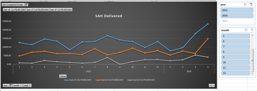
My work was having an issue rolling up and trending out some production and finance information related to output performance and cost, which was making it hard for them to see over a large period of time how they were performing to plan when it came to per unit cost and unit delivery goals. All the information needed for this existed already,  but (and I’m sure this is a big but for a lot of businesses) the information resided in multiple locations and formats making it extremely time consuming to pull together into a cohesive format.

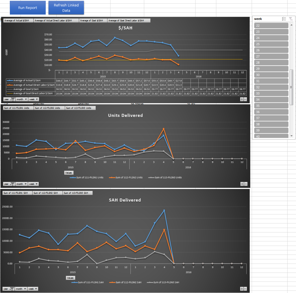
My goal for the dashboard was to create a single location where both the production and finance team could look at together to see how well the company is performing to plan on a weekly/monthly/quarterly basis.

The first part of this project was identifying what information is being used by the two departments:

Finance:

• Monthly overhead costs
• Direct labor cost broken out by factory
• Indirect labor cost broken out by factory

Production:

• Number of units completed by factory
• Number of standard allowed hours (SAH – how long it should take to complete a unit) completed by each factory

The second part was to find the overlapping information that both Production and Finance teams are measuring themselves against, which in our case was:

• $/unit
• $/SAH
• Direct Labor Cost / SAH – this shows how much money we end up spending on labor over a time period versus how long it should generally take to complete the labor

Once I had a chance to look through how the teams currently use and create the reports that are generated for Production and Finance teams, I start looking into where the information was being pulled from.

On the Production side, a new ERP system (Dynamics AX) has all of the information related to finished goods completed form each production location while Finance uses ADP to manage costs related to Production. My goal was to combine these two locations of information and minimize and changes required by the users in each department. In order to accomplish this task, I had to link into the workbook used by Finance to track biweekly spending and pull information for the transaction log in AX. After getting the data pulled into a single location, I needed to change it into a usable format. I accomplished by creating three separate tables:

Financial table

• rolled up all of the direct and indirect labor between all factories
• tied in overhead costs
• added 10% payroll tax adder

Production table

• rolled up daily output into weeks due to all finical data only having visibility down to the week
• pulled in SAH information for the styles being made in each factory
• Rolled up total production unit output and SAH output

Combined table

• This table houses the calculations to show $/SAH and $/Unit on a weekly basis

I created Pivot charts off of the Combined table to show the performance overtime and created two macros to pull the information, refresh the tables, and validate against double counting of unit output.

Attached is an example with some salted data sets the pretty closely represents what we ended up using at filson.

-jess

Beta1.5-Finance-scorecard.xlsm

Leather is a highly variable product due to the inconsistency in size, shape, and quality. These variables are also what makes leather a really unique product to work with, but can also lead to large waste factors and increasing cost for a company.

In order to reduce variability in leather consumption/usage and more accurately track how much leather is on hand, I separate the two ways the leather presents its self as a raw materiel in a typical production house:

• Whole hide (untouched from the tannery)
• Scrap or drop off from blocking

Having two high level buckets makes it easier to understand how usable leather square footage you have on hand is. Think about it this way, if you have 1000 sq. ft. of leather on hand but it’s all in 1 sq. ft. pieces, the belt demand for leather is 500 sq. ft. total but each individual belt requires a 48″ by 1″ piece of leather. You can make exactly 0 belts with the leather you have on hand in it’s current form.

With the buckets above, we create visibility on what form the leather is in, which will help eliminate orders issued for unusable raw material.

The first step in creating the whole hide and scrap locations is to do a cycle count on the leather that’s on hand. Whole hides come in with the size of the hide printed on the flesh side, which can be added up to get an accurate count of how much square footage is available in whole hide form. Getting an accurate count of scrap leather (the drop off leather after the initial cuts of the whole hide) is much more difficult. The easiest way to tackle this with some level of accuracy is the following:

1. Make sure all of the leather types are separated out into their own storage bins
   • grab a weight for each of the empty bins used to store the leather
2. Cut samples of 1 sq. ft. of all of the different leather types and measure the weight
   • if you have a whole hide available for all the different leather scrap, grab a weight for these and calculate the lbs/sq. ft.
3. Weigh the bins each of the different leather types
   • subtract out the weight of the empty bins from the total weight
4. use the lbs/sq. ft. you calculated from step 2 to identify an approximate number of square footage there is in each bin of scrap.
   • Please note that Leather has a high variability in density which makes the weight inconsistent on a square footage basis, if you have enough samples in weight from step 2, you can build out a distribution of how much leather you have based on weight and use the average for the sample. I have found there is about a 30% swing in square footage when using weight to identify square footage and in order to avoid over reporting leather available in scrap, I always use the lower quantile of leather square footage available based on weight.
5. Use the attached tracking sheet when you pull leather from the whole hide location for an order
   • the tracking sheet is standardized so that you mark down
     • the grade of the hide
     • the size of the hide
     • the dimensions of the cut you took out of the hide
6. Place the drop off into your dedicated leather bin based on the type of leather
7. Use the attached calculator to tell you how much leather to consume out of the whole hide location and move into the scrap location.
   • the calculator will roll up the number of whole hides used and their size, the dimensions of the leather cut out, and the remainder available to be placed into the scrap location

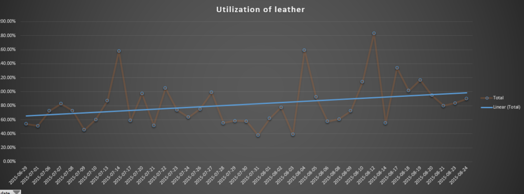
Doing this simple bucketing technique, Filson was able to improve their on hand accuracy of leather from 47% – 80% and also improve the yield on leather (due to better oversight on how much leather is being used from the whole hide location) used on the classic briefcase (70256) from 67% to 88% leather utilization, which can be seen in the graph below:

Leather Consumption calculator

leather block size template

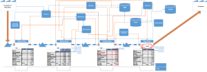
The ultimate goal of a current state value stream map(VSM) is to create a visual representation of how the value object flows through a system in, it should be pretty obvious, its current state. This visual representation should be able to help you visualize where in the process a bottleneck/issue are occurring. The problem is how do you show a current state VSM and what areas are having issues to a person or group who have never seen a VSM? They can be easily overwhelmed by the amount of information being displayed on a VSM and potentially get caught up on other details instead of what they should be focused on, like what are the current areas of opportunity within the value stream. Here’s an example of what a complete current state VSM can look like: : If you’re reading this, you can probably tell where the main issues are occurring, but for someone new, this looks like a complete overwhelming mess so let’s make this more consumable.
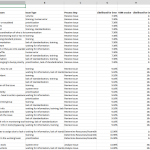
The first thing we need to do is add all of the pain points into from the VSM into an excel sheet and separate them so there is a single pain point per row. Next, we need to type the name of the process step the painpoint relates to in column b.
At this you point you can continue on using only the paint points count to produce the graphs or, if you begin to notice that a lot of the pain points have several issues associated with them, you can break these pain points down into the different issue “buckets” – this can become more of a qualitative art than data science since though so sticking with the defined pain points might be the best bet.
Once you have the pain points and process steps placed in the columns, the next step is to attach a few more elements to the process steps (quality, cycle time, inventory, etc). In the example I have added in the quality comparison (likelihood for error observed vs defined in the VSM session) each process step has a quality number attached to it so in the column next to process step, place the quality number for the associated process step. The quality number will be repeated multiple time like so:: example:: don’t worry, this wont be counted in the graph, it just makes it easier to create a pivot chart. Here is an example of what a completed excel data sheet will look like:

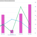
Once you have the data setup, highlight the data and add in a pivot chart. Once the pivot chart has been added, drop the process steps feild choice into the “Axis” category. Next, add in Issue Type, Observation – Likelihood for Error, and VSM session – Likelihood for Error into the “Values” section of the pivot chart fields. We want the Issue Type to be a count and the Observation data to be an average. The next step is to add in a secondary axis in order to scale the likelihood for error data against the count of Issue types. Once you complete those steps, your graph should look like the below:

The graph above makes it much more evident where the bottlenecks or  issues are occurring and should be much more consumable for your customer who need to view the information from the VSM.

Where I work, there are many many internal and external surveys going around and there is always some arbitrary percentage for a target response rate. When I asked why the percentage is set set at certain level, I rarely receive a clear answer and even more troubling is when I ask if any sample size calculations have been done to know exactly how many responses would be needed to to hit a target confidence level and margin of error I get stared at by my like I’m speaking Latin and over complicating a simple task. The problem with that thinking is that we tend to jump to conclusions, based on the survey results, without fully understanding if the changes are due to an actual change in the population that is being surveyed and how easy it is to start doing sample size calculations based on a set confidence level and margin of error.

Without getting too mathy, here are explanations of the two measures that affect the survey results and something that needs to be taken into consideration when comparing surveys (which we can easily do with sample size calculations):
• Margin of error(also known as confidence intervals): the deviation between the results of the respondents and the entire population
o Example: You set the margin of error to 5% for your survey and 90% of survey respondents say they like pizza. A 5% margin of error means that you can be “confident” that between 85% and 95% of the entire population actually like pizza
• Confidence Level: This tells you how often the percentage of the population actually lies within the boundaries of the margin of error.
o Example: between 85% and 95% of the population likes pizza (like above) and we chose a 95% confidence level, we can then say 95% of the time, between 85% and 95% of the population likes pizza.
Alright, at this point you still might be asking yourself “is this important and/or how does this help with survey results?” Don’t worry, I’m going to try and address that more directly below(which is pretty much a TLDR of the example link above (TLDR = Too long, didn’t read)):

Let’s say we have an in-scope deployment group of 500 people.
We send the survey out and only 88 people respond.
If we look at the results and take into account a Confidence level of 95% (there is an equation to do this that I can show you or you can look it up on the interwebs), the margin of error is about 9.5% which means we would need to see a shift (positive or negative) of greater than 9.5% in the survey results before we could truly say there was any change at all in the population.
So if we are comparing two surveys and we see an increase of 8% in understanding of LMS tools but the margin of error is 10% for the survey, there was technically no change at all and that 8% could be attributed to noise and is not representative of the population we are trying to survey.

So how do we easily start calculating required sample sizes and the other mumbo-jumbo above? This is where the internet really come in handy because right here is a hand calculator that not only takes into account confidence level and margin of error, but also the estimated response rate!
If we start using the calculator (here again) to get the sample size, we can start comparing survey results with much more confidence in the fact that employee opinions are changing and we aren’t over processing by looking into opinion changes caused by statistical noise and not actual population opinion shifts.

-jess